MQS Solution on 2-D Trough

Editors： 趙嘉瀅、林俊宏、張峰嘉

Advisor： 江簡富 教授

Demonstration:
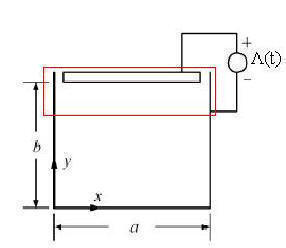
Consider a rectangular trough with the geometry shown in Left Fig. The current
on the side and bottom walls flows in the z direction, and that on the top
wall flows in the − direction. The vector potential satisfies the Laplace
equation inside the trough, namely, ▽²A_z = 0. The boundary conditions
require that A_z(0, y) = A_z(a, y) = A_z(x, 0) = 0 and A_z(x, b) =A , where
is the total magnetic flux per unit length flowing between the top
wall and the other walls. By  MQS approximation:

The Biot-Savart low can be derived as follows：

Thus, the magnetic field intensity H in x and y direction：

Finally, we simulate the distribution of the surface current Js.From the MQS approximation.

The Maxwell's equations governing the magnetic fields are：

Thus, the surface current Js at boundaries：

Js at x=0 , Hy(x=0,y):

Js at x=a , Hy(x=a,y):

Js at y=0 , Hx(x,y=0):

Js at y=b , Hy(x,y=b):