Parallel-Plate Waveguide

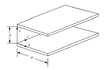
The figure shows two parallel plates of width \(w\) and of infinite length, separated by a distance \(d\). One of the wave solution between these two plates is

\[\bar{E}=\hat{x}E_x\left(z\right)=\hat{x}E_0e^{-jkz}\] \[\bar{H}=\hat{y}H_y\left(z\right)=\hat{y}\frac{1}{\eta}E_0e^{-jkz}\]

Where \(k=\sqrt{\mu\varepsilon}\) and \(\eta=\sqrt{\frac{\mu}{\varepsilon}}\). At \(x = 0\) and \(x = d\), the boundary conditions: \( \hat{n}\times\bar{E}=0 \) and \( \hat{n}\cdot\bar{B}=0 \) are satisfied.

The other boundary conditions: \(\hat{n}\times\bar{H}=J_s\) and \(\hat{n}\cdot\bar{D}=\rho_s\) which imply that

\[\bar{J_s}=\hat{z}E_0{\eta}e^{-jkz} \mbox{ and } \rho_s=\varepsilon E_0e^{-jkz} \mbox{ at }x\mbox{=}0 \] \[\bar{J_s}=-\hat{z}E_0{\eta}e^{-jkz} \mbox{ and } \rho_s=-\varepsilon E_0e^{-jkz} \mbox{ at }x\mbox{=}d \]

The current \(I\) on the bottom plate, and the voltage \(V\) across the two plates, can be defined as

\[I\left(z\right)=\int_{0}^{w}H_y\left(z\right)dy={wH}_y(z)\mbox{ }\mbox{ }\mbox{ }\mbox{ }\mbox{ }\mbox{ }\mbox{ }(1.15)\] \[V\left(z\right)=\int_{0}^{d}{E_x}\left(z\right)dx={dE}_x(z)\mbox{ }\mbox{ }\mbox{ }\mbox{ }\mbox{ }\mbox{ }\mbox{ }(1.16)\]

Note that the current on the top plate is of opposite sign with that on the bottom plate, implying that the currents on both plates flow in opposite directions.

Substituting the field expression into the Faraday's law and Ampere's law, respectively, we have

\[\frac{d}{dz}E_z\left(z\right)=-jw\mu H_y\left(z\right)\] \[\frac{d}{dz}H_y\left(z\right)=-jw\varepsilon E_x\left(z\right)\]

By using the definition in (1.15), (1.16) can be transformed into

\[\frac{d}{dz}V\left(z\right)=-jwLI\left(z\right)\mbox{ }\mbox{ }\mbox{ }\mbox{ }\mbox{ }\mbox{ }\mbox{ }(1.17)\] \[\frac{d}{dz}I\left(z\right)=-jwCV\left(z\right)\mbox{ }\mbox{ }\mbox{ }\mbox{ }\mbox{ }\mbox{ }\mbox{ }(1.18)\]

Where \(L=\frac{\mu d}{w}\) \((H/m)\), \(C=\frac{\varepsilon w}{d}\)\((F/m)\) are unit-length inductance and capacitance, respectively, of the parallel-plate waveguide. Equations (1.17) and (1.18) are called telegrapher's equations or transmission line equations, we have

\[\frac{d^2}{dz^2}V(z)=-w^2LCV\left(z\right)=-k^2V\left(z\right)\mbox{ }\mbox{ }\mbox{ }\mbox{ }\mbox{ }\mbox{ }\mbox{ }(1.19)\]

Since \(LC=\mu\varepsilon\), the solution to (1.19) are

\[V\left(z\right)=V_0e^{\pm j k z} , I\left(z\right)=\mp\frac{1}{Z_0}V_0e^{\pm j k z}\]

\(Z_0=\sqrt{\frac{L}{C}}=\frac{d}{w}\sqrt{\frac{\mu}{\varepsilon}}\) is the characteristic impedance of the transmission line.

Electric Field Distribution and Surface Charge Distribution

Magnetic Field Distribution and Surface Current Distribution