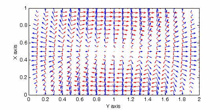
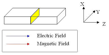
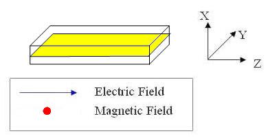
There are two sets of wave modes, TE and TM modes, that can propagate in a rectangular waveguide as shown in the Fig.
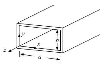
Fig. Configuration of a rectangular waveguide.
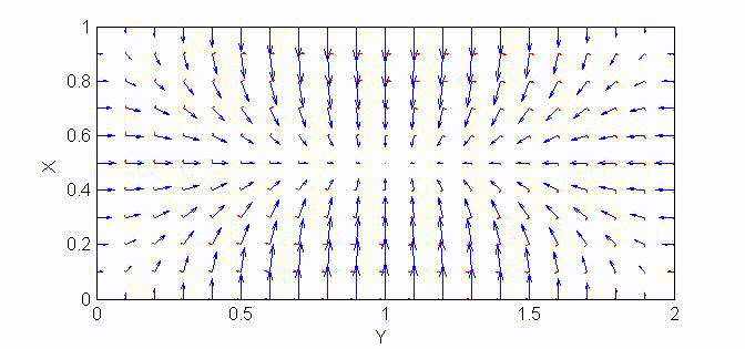
For the TM modes, \(H_z=0\), and the \(E_z\) component takes the form:
$$E_z=A\sin{(k_xx)}\sin{(k_yy)}e^{\mp jk_zz}$$
Substituting this into the wave equation gives the dispersion relation: $${k_x}^2+{k_y}^2+{k_z}^2=\omega^2\mu\epsilon$$
The boundary conditions require that \(E_z=0\) at \(x=a\) and \(y=a\). Therefore, the guidance conditions are obtained as $$k_x=\frac{m\pi}a,\;k_y=\frac{n\pi}b,\quad\textrm{where }\;m,n=1,2,3,...$$
The TM mode with \(k_x=m\pi/a,\;k_y=n\pi/b\) is called the \({\rm TM}_{mn}\) mode.
The other components of the electromagnetic fields can then be derived from \(E_z\) by field decomposition method:
$$\begin{aligned}\overline{\bf E}_s&=\frac1{k_x^2+k_y^2}\left(-j\omega\mu\nabla_s\times\overline{\bf H}_z+\nabla_s\frac{\partial E_z}{\partial z}\right)=\frac{-j\omega\mu}{k_c^2}\nabla_s\frac{\partial E_z}{\partial z}\\
\overline{\bf H}_s&=\frac1{k_x^2+k_y^2}\left(j\omega\epsilon\nabla_s\times\overline{\bf E}_z+\nabla_s\frac{\partial H_z}{\partial z}\right)=\frac{j\omega\epsilon}{k_c^2}\nabla_s\times\overline{\bf E}_z\end{aligned}$$
where \(\overline{\bf E}_s:=\hat{x}E_x+\hat{y}E_y\), \(\overline{\bf H}_s:=\hat{x}H_x+\hat{y}H_y\), \(\overline{\bf E}_z:=\hat{z}E_z\), \(\overline{\bf H}_z:=\hat{z}H_z\), \(\nabla_s:=\hat{x}\frac{\partial}{\partial x}+\hat{y}\frac{\partial}{\partial y}\).
The result of the derivation is given below.
| Table. Field Expressions and Associated Parameters for TM Mode in a Rectangular Waveguide | |
|---|---|
|
\[\begin{aligned}H_z&=0\\ E_z&=A\sin\frac{m\pi x}a\sin\frac{n\pi y}be^{\mp jk_zz}\\ E_x&=\mp j\frac{\lambda_c^2}{2\pi\lambda_g}\frac{m\pi}aA\cos\frac{m\pi x}a\sin\frac{n\pi y}be^{\mp jk_zz}\\ E_y&=\mp j\frac{\lambda_c^2}{2\pi\lambda_g}\frac{n\pi}bA\sin\frac{m\pi x}a\cos\frac{n\pi y}be^{\mp jk_zz}\\ H_x&=\mp\frac{E_y}{\eta_g}\\ H_y&=\pm\frac{E_x}{\eta_g}\end{aligned}\] |
\[\begin{aligned}f_c&=\frac1{2\sqrt{\mu\epsilon}}\sqrt{\left(\frac{m}a\right)^2+\left(\frac{n}b\right)^2}\\ \lambda_c&=\frac2{\sqrt{(m/a)^2+(n/b)^2}}\\ \lambda_g&=\frac{\lambda}{\sqrt{1-(\lambda/\lambda_c)^2}}=\frac{\lambda}{\sqrt{1-(f_c/f)^2}}\\ v_{pz}&=\frac1{\sqrt{\mu\epsilon}\sqrt{1-(f_c/f)^2}}=\frac1{\sqrt{\mu\epsilon}\sqrt{1-(\lambda/\lambda_c)^2}}\\ \eta_g&=\sqrt{\frac\mu\epsilon}\sqrt{1-\left(\frac{f_c}f\right)^2}=\sqrt{\frac\mu\epsilon}\sqrt{1-\left(\frac{\lambda}{\lambda_c}\right)^2}\end{aligned}\] |