Transmission Line Connected with a Nonlinear Load

Authors: 陳品諺、李佾儒

Advisor: 江簡富教授

Load-line technique is a graphical technique frequently used to analyze the voltage and current along a transmission line connected with a nonlinear load.

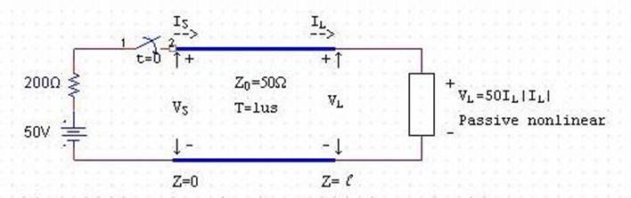
Fig.1: Transmission line terminated by a passive nonlinear element and driven by a constant voltage source in series with a resistance.

Fig.1 shows a transmission line terminated by a passive nonlinear element having the I-V relationship of , and the source end is consisted of a resistor of 200Ω and a dc voltage of 50V. The characteristic impedance of the transmission line is, and the transverse time along the line is. The switch S is closed at, and the load-line technique is used to obtain the time variation of the voltages and at the source and at the load ends, respectively.

The Kirchhoff voltage law at implies

At ,

 and  are the voltage and current, respectively, of the (+) wave propagating in +z direction immediately after closure of the switch. We can solve  and  graphically by drawing two straight lines to represent (1) and (2) as shown in Fig.2. The point of intersection is denoted by A, which gives the values of  and.

When the (+) wave reaches the load end at, a (-) wave is induced, the voltage and current at at can be expressed a

            where  and I^- are the (-) wave voltage and current, respectively. The solution of  and  is given by the intersection of the curve representing (3) and the straight line representing (4), the intersection is denoted by B.

            When the (-) wave reaches the source end at, another reflection is induced, denoted as (-+) wave.  

            The voltage and current at and satisfies the same KVL:

The voltage and current are consisted of 

　

            where  and  are the (-+) wave voltage and current, respectively. Note that  and is a solution to (5), implying that the straight line representing (6) passes through B. Thus, the solution of (5) and (6) is given by point C in Fig.2. 

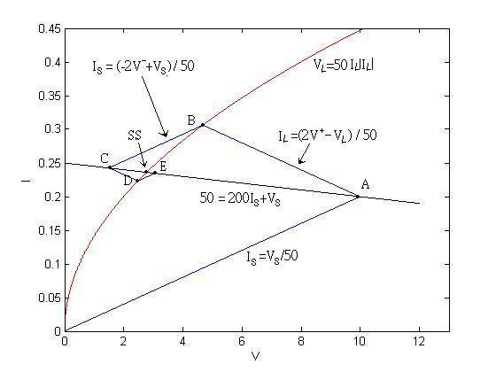
Fig.2: Graphical representation of voltage and current waves.

            Continuing this process, we observe that the solutions at are the points of intersection of either the source or the load V-I curve with the straight lines of slope  or, respectively. The first straight line launches at the origin and the following straight line originates at the previous point of intersection. To be more specific, solutions of  and  are obtained by drawing the intersection of the straight lines of slope  and (1), whereas that of  and  are obtained by drawing the intersection of the straight lines of slope  and (3), originating from A, and so on.

            Once we have the time variations of  and ； and, the voltage and current at an arbitrary point on the transmission line at time t can be obtained. Consider the following example. When at, the voltage and current should be equal to that at the load end when. On the other hand, at the same time, at, the (-) wave has not yet traveled to this point, hence the voltage and current is equal to that at the source end when.